How To Delete Pivot Table?

The Pivot Table function in Excel is a fantastic time-saver. Quickly summarise thousands of rows of data with no knowledge of formulas or coding. The only skills required are the ability to use the mouse and a basic understanding of how to make a Pivot Table.

Here I will demonstrate several approaches to removing Pivot Tables from Excel.

Excel’s Pivot Table Deletion Guide

Since you’ve found this post, I’ll assume you already have one or more Pivot Tables set up that you’d like to get rid of.

There are several options for removing a Pivot Table. How you opt to get rid of the Pivot Table will determine which approach you take.

Here are some examples of the kinds of situations I’ll be discussing in this guide:

1. Get rid of the pivot table and the information it generated (the summary created using the Pivot Table)
2. Get rid of the pivot table, but save the information it generated.
3. Get rid of the extra information while keeping the Pivot Table.

Let’s go right in and check out how each of these works.

Get Rid of the Pivot Table and the Data It Produced.

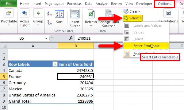
Please see the attached Pivot table example, which I used to calculate the total revenue earned across multiple geographic areas (to which I will be referring to as Pivot Table summary data in this tutorial).

Here’s how to get rid of that Pivot table and all that summary information forever:

1. In the Pivot Table, pick any cell and click “Show Data.”
2. To access the Analyze section of the ribbon, select it. When you choose a cell in the Pivot Table, a new contextual tab will emerge.
3. Select may be found in the Actions menu.
4. All of the Pivot Table can be viewed by selecting it. When you do this, the entire Pivot table will be highlighted.
5. Press the delete key.

With those commands in place, the Pivot Table would be removed.

If you don’t want the Pivot Table anymore, you can also just delete the worksheet it’s on. You should not do this if the worksheet contains any additional information.

Do Away With the Pivot Table, But Save the Data it Generated.

In some circumstances, you may wish to remove the Pivot table yet retain the data that was derived from it. This may be the situation if you’ve utilised a Pivot Table and now wish to provide your boss/client simply the data that resulted from your analysis.

Another time this can be necessary is if your Pivot Table is taking up too much room on the worksheet. Eliminating such a Pivot table can have a significant impact on the overall size of an Excel file.

I want to preserve the data in cells A3:B8 but hide the Pivot Table, as shown in the following example.

Here are the measures to take:

1. In the Pivot Table, pick any cell and click “Show Data.”
2. To access the Analyze section of the ribbon, select it. When you choose a cell in the Pivot Table, a new contextual tab will emerge.
3. Select may be found in the Actions menu.
4. All of the Pivot Table can be viewed by selecting it. When you do this, the entire Pivot table will be highlighted.
5. To use the context menu, right-click on a Pivot Table cell.
6. Simply select the Copy option. By clicking this, you may replicate a complete Pivot Table.
7. Access the main menu by selecting the “Home” option.
8. Pick the Paste menu item.

Select the first icon labelled “Paste Values” to begin pasting values (which is of Paste as Value).

The methods outlined above would remove the Pivot Table without affecting the final data.

Here are some useful keyboard shortcuts:

• A Pivot Table can be selected in its entirety by selecting any cell in the table and then pressing “Control + A” on your keyboard.
• Once you have copied all of the data from the Pivot table, you can paste it as values by pressing ALT+E+S+V+Enter (one key after the other)

The techniques mentioned above can also be used to copy data from a Pivot Table and paste it as values elsewhere (either inside the same worksheet or in a different worksheet/workbook). The Pivot Table can be removed after the information has been collected.

Remove the Accumulated Information But Always use the Pivot Table

We’ll pretend you’ve made a Pivot Table and summarised the data (selecting the columns and rows you’re interested in using filters and headings) in the way depicted in the table below.

You can also choose to preserve the Pivot Table but discard the data it contains in order to reorganise the information and generate a new summary.

You can delete the Pivot Table along with the data if you select it and then press the delete key.

Listed here are the manoeuvres to be taken in order to retain the Pivot table while discarding the output data:

1. In the Pivot Table, pick any cell and click “Show Data.”
2. To access the Analyze section of the ribbon, select it. When you choose a cell in the Pivot Table, a new contextual tab will emerge.
3. Select “Clear” from the Actions menu.
4. Select “Clear All” from the drop-down menu.

Conclusion

I think we’ve reached the end of this discussion. The many Excel Pivot table deletion options are as follows. Applying these methods going forward will make working with Excel much simpler.

Please let us know if you have any further questions about this or any other Excel function below. As always, we’re here to lend a hand.